For the same flexible microstrip, insertion loss drops noticeably after changing to another process, yet the report directly states, “the copper surface is smoother, so loss is reduced.” This conclusion may be too hasty: if the copper conductor cross-section, adhesive layer, and surface condition all changed together, the improvement of the entire process cannot be attributed entirely to one factor. Reading a loss report is not just about finding the lower curve;
For the same flexible microstrip, insertion loss drops noticeably after changing to another process, yet the report directly states, “the copper surface is smoother, so loss is reduced.” This conclusion may be too hasty: if the copper conductor cross-section, adhesive layer, and surface condition all changed together, the improvement of the entire process cannot be attributed entirely to one factor. Reading a loss report is not just about finding the lower curve; it is also about judging what variables the comparison actually isolated. In a 2022 flexible microstrip study, Woo et al. provided both cross-section scans and physical measurements, which is a good case for practicing this kind of judgment.
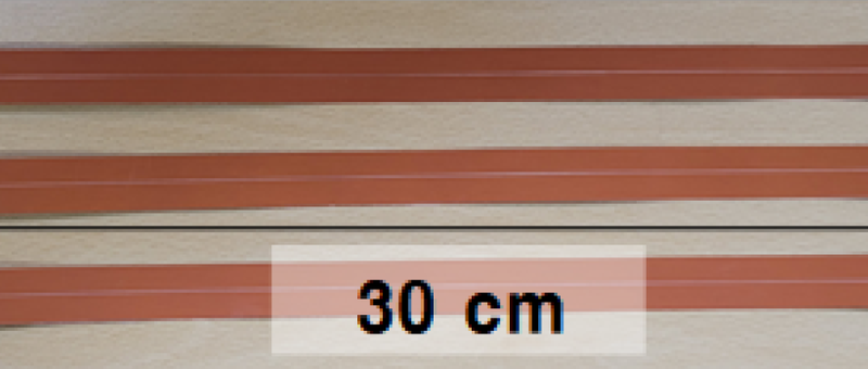
Figure 1: Local view of a conventional-process flexible microstrip sample used for insertion loss comparison.
First Look at the Cross-Sections: The Two Photos Already Expose the Variables
Figure 2 is not a simple comparison of “rough copper vs. smooth copper.” The bottom surface of the conductor in the left sample has obvious undulations, while the right sample is not only smoother but also has a cross-sectional profile that becomes arched. If you only circle the rough surface while ignoring the profile change, you lose another factor that may affect loss at the very first step of reading the image.
High-frequency conductor loss is related to how current is distributed. Surface condition affects current transmission on the conductor surface; sharp corners and arc-shaped profiles of the cross-section also change local current concentration. Both effects may contribute to the result, but “may contribute” and “have already been separately quantified” are not the same conclusion. With different actual copper foils, frequencies, and stack-ups, the magnitude of the effect will also vary.
When annotating the report, first write down the facts that can be confirmed from the photos: different surfaces, different profiles. Then list items that cannot yet be confirmed from the photos as items to be checked, such as roughness measurement metrics, sampling locations, and statistical scope. You cannot make a quantitative conclusion for an entire roll of copper foil based on one localized electron microscope image.

Figure 2: Copper conductor cross-sections of the two processes: the left bottom surface is rougher, while the right simultaneously shows a smoother surface and an arched profile.
Treat the Shape Sweep as a Separate Ruler
The authors use α to represent the ratio of the bottom linewidth to the top linewidth. When α equals 1, the shape is close to rectangular; as α decreases, a more pronounced arch forms. This parameter is important: it turns “looks a bit rounder” into a scannable geometric input, making it convenient to observe the changes caused by shape within the same simulation framework.
In Table 2 of the original paper, at 10 GHz, as α changes from 1 to 0.26, the loss per unit length changes from 0.266 to 0.235 dB/cm, a difference of 0.031 dB/cm. This set of numbers answers the question of the impact of cross-section change in that model. It is not a universal benefit for all laminates, nor can it be used to directly promise how much channel loss a certain high-speed board can reduce.
Figure 4 gives the corresponding current density simulation: local concentration is more obvious for the rectangular cross-section, and the distribution changes for the arched cross-section. Here one should say “the model supports that shape affects current distribution,” not “the instrument has measured current flowing along this color.” Contour plots and measured curves have different evidentiary natures and should also be labeled separately in the report.
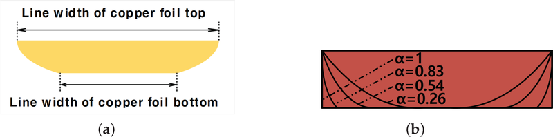
Figure 3: The cross-section parameter α is the ratio of bottom linewidth to top linewidth; reducing α changes the cross-section shape.
The Physical Improvement Is Larger—Do Not Rush to Assign Credit
In the physical measurements, the unit-length insertion losses of the two types of 30 cm samples at 10 GHz are approximately 0.66 and 0.37 dB/cm, respectively. This change is clearly larger than the earlier cross-section sweep difference, but one cannot infer from this that “the remaining part must all come from roughness.” Between the model and the sample, there is not just one unknown variable.
Table 3 of the original paper also lists structural differences: the adhesive layer configurations of the two process samples are not the same. The dielectric environment participates in the electric field distribution and also affects loss. Therefore, what the measurement proves is that these specific samples and their complete structures differ under those test conditions, not that the respective contributions of roughness, cross-section, and adhesive layer have been separated.
The authors also point out that the loss tangent used in the model came from a 2 GHz measurement but was applied to a higher frequency band, which may contribute to the discrepancy between simulation and measurement. Readers need not reject the entire study because of this; the correct approach is to retain its valid comparisons while narrowing the scope of the conclusions. A model can explain trends, but that does not mean the absolute values at every frequency point have been closed.
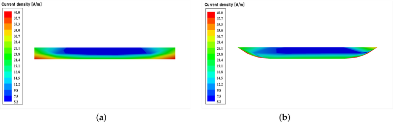
Figure 4: Current density distribution simulated at 10 GHz: the degree of local concentration differs between rectangular and arched cross-sections.
Review with a Two-Column Table
The next time you receive A/B insertion loss reports, first list side by side the trace length, trace width, copper thickness, cross-section profile, roughness metrics, dielectric and adhesive layer, test frequency band, calibration, and transition structure. Check the same items; circle the different items separately. If you circle three or four items at once, write the conclusion as an “overall scheme comparison,” not as “determined by one material parameter.”
Also align the vertical-axis basis: is it dB for the entire channel, or normalized dB/cm? Have connector and transition losses been handled? You cannot simply divide the total loss of a short line including transitions by its length and consider that you have obtained a transmission-line loss fully comparable to that of a long line. If the conditions are not aligned, even standardized units may mislead the selection.
If the goal is only to select a usable process, a complete scheme comparison can be valuable; if the goal is to optimize a certain parameter, additional single-variable samples or a validated model are needed. First clarify whether you are doing selection or attribution, and only then will you know whether the existing report is sufficient.
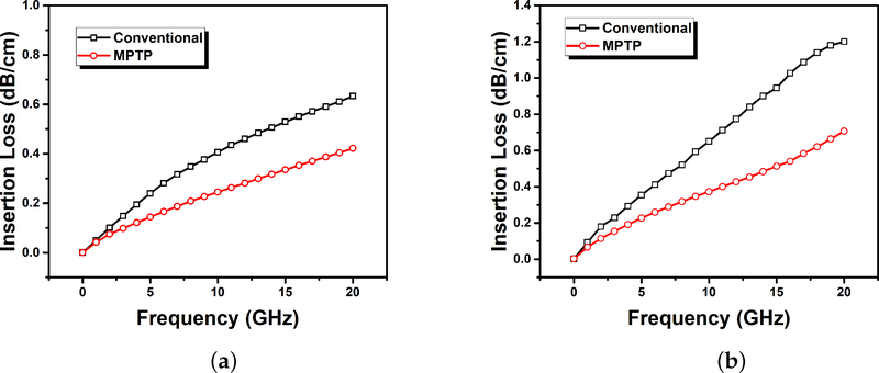
Figure 5: Comparison of insertion loss per unit length for the two processes: left is simulation, right is measurement; the two sets of curves cannot be mixed as the same type of evidence.
The ability to read loss reports is reflected in knowing what each curve can prove and cannot prove. In the next review, first make a two-column condition table, then divide the conclusions into “model single-variable results” and “physical overall results.” Do not rush to assign all the credit to one factor; are the two curves you are comparing changing only the copper surface, or have the cross-section and stack-up also changed together?
About Maxipcb
Maxipcb empowers innovators to turn cutting-edge technologies into reality.We offer one-stop solutions for design, simulation, testing, PCB manufacturing, component procurement and SMT assembly, enabling efficient development, rapid deployment and risk control across the full product lifecycle.
Serving the world in communications, industrial automation, aerospace, automotive, semiconductor and beyond, we build a safer, more connected future together.
