
Signal integrity (SI) problems in high-speed PCBs are usually not caused directly by schematic errors, but are jointly determined by routing topology, via layer-transition strategy, and stack-up material selection. Continuous reference planes, adjacent stitching vias, reasonable control of via stubs, and material selection based on Dk and Df are key to reducing return-path discontinuity, via resonance, signal loss, crosstalk, and EMI risk.
Signal integrity failures are rarely triggered by a single major mistake; more often, they accumulate from a series of seemingly reasonable layout decisions. For example: choosing a certain via type, routing a differential pair through several layer transitions, or using a default stack-up material—each of these decisions changes the electrical behavior of the signal. By the time the engineer runs analysis or completes the first prototype board, the combined effect of these decisions manifests as timing failures, excessive noise, or eye-diagram failures.
The root cause almost always lies in PCB layout, not in the schematic. The schematic defines which signals connect to which pins; the layout determines the electrical behavior of those connections. The three layout decisions with the greatest impact on signal quality are: routing topology, via strategy, and stack-up material selection.
Why Is “Return Current” Both Practical and Potentially Misleading?
Most articles on signal integrity in PCB layout describe return current as current flowing from the receiver back to the source on a reference plane. This description is easy to understand and provides engineers with a practical mental model that is sufficiently reliable for most layout decisions. However, it is a simplification, and in the boundary cases where signal integrity problems are most likely to occur, this simplification may no longer hold.
From a physical perspective, a signal is an electromagnetic wave propagating through the dielectric between a trace and the nearest conductive structure it can find (usually the plane below the signal trace). The propagation speed of the wave is determined by the local dielectric constant: approximately the speed of light in air at the PCB surface, and approximately half the speed of light in standard FR-4 with a Dk of 4.0–4.2.
As the electromagnetic wave propagates forward, the electric field terminates on any copper it can reach. Electrons in the copper respond to the field by moving. The “current” measured on the reference plane is actually the conductor’s response to the field, not an independent entity with a destination.
Even if two copper layers are physically separated from each other, the electromagnetic field does not stop propagating because of this. The dielectric fills the space between them, allowing the field to pass through. The field propagates wherever the geometry allows and induces current on every conductor it touches.
This perspective is important because it explains failure modes that the statement “return current will find another path” cannot clearly explain.
When there is a gap in the reference plane, the field does not stop at the gap; it expands to any conductor it can find and terminates on that conductor. Usually, this conductor is the adjacent plane below. Energy couples through the gap, propagates between the upper and lower planes in a parallel-plate mode, and induces current on the lower plane. The current observed on the lower plane is not a “lost” return current, but the conductor’s response to the field escaping its intended boundary.
When a signal via transitions between layers and there is no nearby ground via, the electromagnetic field must cross between reference planes. Without a ground via providing a continuous boundary, the field spreads in the inter-plane region and induces current on any copper it touches, increasing the loop area. The current distribution on the lower plane appears chaotic because, when the boundary conditions of the field are unconstrained, the electromagnetic field continues to spread until it couples to a conductor where it can terminate.
Stitching vias provide a continuous conductive boundary when the electromagnetic field crosses reference planes, thereby limiting the spread of the field, making the induced current distribution more concentrated, and reducing the loop area. Whether this mechanism is described as “return current flowing along ground vias” or “the field having a continuous boundary at the transition,” the physical essence is the same. The field perspective more clearly explains why stitching vias are effective.
Decision 1
Routing Topology Determines Signal Propagation Behavior
Every high-speed signal propagates along a transmission line as a wave and passes through dielectric material (such as radio waves and infrared). The wave requires two elements: a forward path (the trace) and a reference conductive structure, usually called the “return path.”
However, a more accurate expression is “adjacent path” or “reference path.” There is no situation in which current “returns” from one conductor to another, because electrons do not jump from one conductor to another.
In almost all PCB layout situations, the best reference path is a large, complete layer of conductive material that is very close to the transmission-line trace (i.e., the signal trace) in the Z-axis direction of the PCB, separated only by a thin dielectric material.
The electromagnetic field preferentially couples to the adjacent reference plane, and the return current is pulled along the plane by the field between the trace and that plane. Directly under the trace is usually the path of least impedance, so the current distribution concentrates under the trace. This is how electromagnetic energy propagates in a PCB.
Comparison of return paths for different PCB routings:
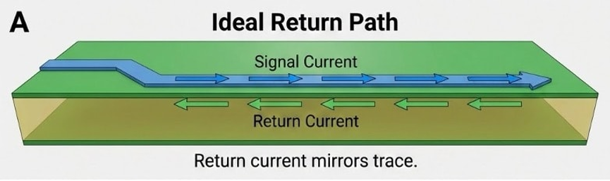
A. Ideal return-path geometry, forming an adjacent return path through tightly coupled displacement current.
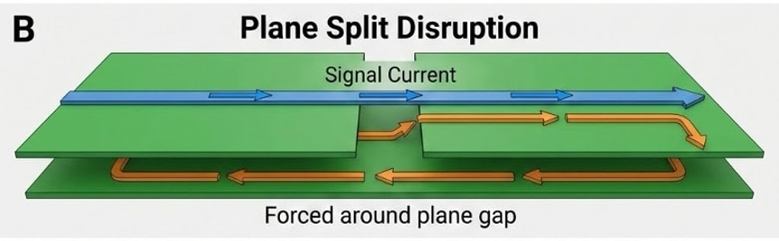
B. A gap in the adjacent plane causes the field to take a longer path to the adjacent return plane.
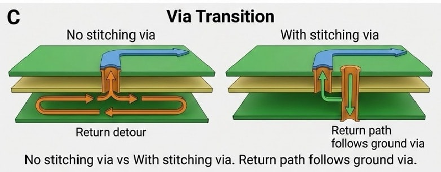
C. How return-path stitching vias affect the return path.
When a signal changes layers through a via, the return current must also change reference planes. If there is no nearby ground via to provide this transition, the return current must find another path. The return current spreads out, travels farther, and increases the loop area. An increased loop area increases the inductance of the signal path. Inductance slows edge speed, creates voltage spikes, and increases electromagnetic radiation.
This is a routing topology problem. Two differential pairs on the same circuit board, even with the same stack-up and the same driver IC, may have completely different signal quality due to different routing. A differential pair located on only two layers and changing reference plane only once will have a clean return path. A differential pair spanning nine layers and four reference planes will have a return path riddled with discontinuities.
The Sigrity X Aurora return-path analysis workflow can visually highlight problems in the design. In the test design, two USB differential pairs are routed on the same circuit board. The first differential pair (P0_USB) changes two layers and maintains a clean, high-quality return path. The second differential pair (P1_USB) crosses four reference planes and changes nine layers before returning to the top layer. The return-path quality differs greatly between these two circuits, even though both pass DRC; it is the routing decisions that cause the difference.
Decision 2
Via Type Determines the Frequency Ceiling of the Signal
When a signal transitions from one layer to another through a plated through-hole (PTH) via, the via extends through the entire board thickness. The portion of the via below the target layer is called a stub. A stub is an open-ended conductor; although it is not part of the effective signal path, electromagnetic energy still couples into it.
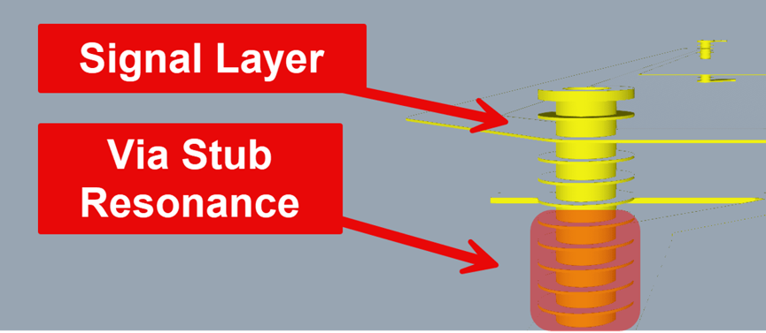
Conceptual diagram of via stub resonance. The cross-section shows a PTH via with the stub portion below the target signal layer highlighted; removing these stubs can reduce the problem of EMI field effects spreading arbitrarily.
Energy propagates down the stub, reaches the open end, and reflects back. At a specific frequency, the round-trip delay of the signal in the stub equals half the signal wavelength. At that frequency, the reflected energy cancels the original signal. This forms a resonant dip in the frequency response, meaning the signal suffers power loss exactly at that frequency.
The frequency at which this occurs depends on the stub length, the dielectric constant (Dk) of the board material, and the complete 3D geometry of the via structure (pad size, antipad spacing, ground via distance). A longer stub resonates at a lower frequency. Higher Dk also lowers the resonant frequency because the signal propagates more slowly in a material with a higher dielectric constant. In Advanced Signal Integrity for High-Speed Digital Designs (Hall et al.), a full-wave 3D electromagnetic simulation of a 37.8 mil via stub shows resonance at approximately 10 GHz.
At that resonant frequency, about 62% of the signal power radiates to the surrounding plane layers rather than reaching the receiver. The authors note that a simple quarter-wavelength formula can only roughly approximate the actual resonant frequency (with an error in the range of several GHz), because the parasitic capacitance and inductance of the physical via structure shift the resonance point. This conclusion has practical significance: if the signal bandwidth approaches the stub’s resonant frequency, the stub should be shortened or removed.
This is why via type is critical. Blind vias, buried vias, and back-drilled vias can reduce or remove stubs. A blind via connecting Layer 1 and Layer 3 has no stub below Layer 3. For a back-drilled PTH via, the stub is physically removed after plating is completed. Selecting the appropriate via type according to signal frequency determines the upper limit of the usable channel bandwidth.
Decision 3
Stack-Up Material Selection Determines Signal Speed and Transmission Loss
Stack-up material affects every signal on the board. Two properties are most critical: dielectric constant (Dk) and dissipation factor (Df), the latter also called loss tangent.
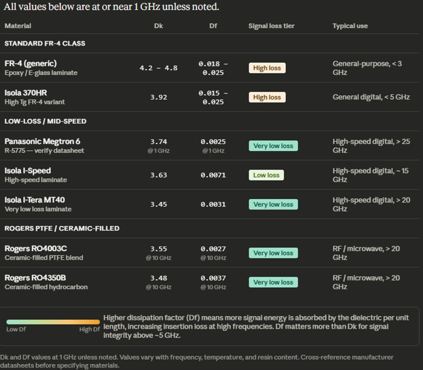
The material comparison table lists approximate Dk and Df values for FR-4, Megtron 6, Isola I-Speed, and Rogers materials from multiple sources. The data is for reference only and must not be used for design. Specifically for Panasonic Megtron 6, material parameter values may differ because its specifications are frequently updated. Before specifying a material, verify all values in this table with the manufacturer. Cadence assumes no liability for design errors caused by failure to verify the above information with the manufacturer in the specific application scenario.
Dk controls signal speed and impedance. Higher Dk reduces signal speed and changes the impedance relationship between trace width and dielectric thickness. If the material is changed from FR-4 (Dk approximately 4.0) to a low-loss laminate (such as Panasonic Megtron 6, Dk approximately 3.63), the impedance will change under the same trace geometry. The trace width needs to be recalculated for the new material.
Df controls signal loss at high frequencies. Each time the signal wave passes through the dielectric, some energy is absorbed and converted into heat. The higher the Df, the greater the loss per unit length, and the loss increases with frequency. Standard FR-4 (Df approximately 0.015 to 0.025) is suitable for signals up to a few GHz. For higher-speed signals, low-loss materials such as Isola I-Speed (Df approximately 0.007) or Megtron 6 can significantly reduce attenuation.
Dk also affects crosstalk. Low-Dk materials can reduce coupling between adjacent traces. Sierra Circuits’ HDI Design Guide states that in high-density interconnect (HDI) substrates, using low-Dk materials and shortening the length of coupled traces can reduce crosstalk by up to 50%.
Material selection only needs to be made once in the cross-section editor, and it propagates to every impedance calculation, every loss simulation, and every crosstalk analysis for the entire board.
Layout Decisions, Not Schematic Decisions
The schematic does not specify via type, routing layer transitions, or board material; these are all layout decisions: they determine whether the signal arrives intact or degraded. Routing topology determines return-path quality, via strategy determines the frequency ceiling, and material selection determines the loss floor and crosstalk baseline.
Each of these decisions can be evaluated during layout using Allegro X PCB Designer and Sigrity X Aurora. Before releasing the design to manufacturing, you can extract routing topology, simulate via structures, and verify material properties. The core principle is: make design decisions based on analysis data, not on default settings. Click “Read Original” at the end of the article to read the e-book and learn how to optimize the complete workflow in high-speed PCB design to achieve high-performance signal integrity.