The difficulty of tuning the RF front-end lies in these invisible "hidden parameters". Today, we will talk about these two easily overlooked key points.
Is the RF front-end difficult to tune? Impedance matching and copper clearance determine success or failure
A Troublesome Debugging Scene
Last month, I helped a friend check the design of a 2.4GHz WiFi module. The schematic was correct, and the component selection was reasonable, but the sensitivity was 8dB lower than the datasheet specification. Modules from several manufacturers were replaced, and the results were similar. Finally, it was found to be a PCB routing problem—the copper clearance on both sides of the RF trace was too close, which "ate up" the impedance.
To be honest, I have seen this situation too many times. Many engineers have a misunderstanding in RF front-end design: they think that selecting the right components and drawing the correct schematic is enough. In fact, in RF PCB design, the two details of impedance matching and copper clearance often determine success or failure.
The difficulty of tuning the RF front-end lies in these invisible "hidden parameters". Today, we will talk about these two easily overlooked key points.
Impedance Matching: The "Life-or-Death Line" of RF Design
First, let’s talk about impedance matching, which is the core of RF design. When an RF signal propagates on a transmission line, reflection occurs if impedance mismatch is encountered. The reflected signal and the incident signal superimpose to form a standing wave, resulting in signal distortion and reduced power transmission efficiency.
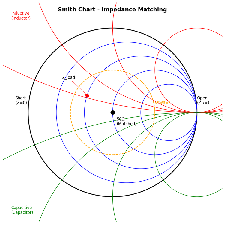
Figure 1: Smith Chart - Graphical Tool for Impedance Matching
Let’s take an intuitive example: a 50Ω transmission line is connected to a 75Ω load, the reflection coefficient is 0.2, and the return loss is about -14dB. This means 4% of the power is reflected back. Does it sound small? But in an RF system, this 4% may mean the communication distance is shortened by half.
Key Indicators You Must Understand
Three main indicators are used to evaluate the quality of impedance matching:
- Return Loss (RL): The power ratio of the reflected signal to the incident signal, in dB. The more negative the value, the better. Generally, it is required to be ≤-15dB, and high-quality designs require ≤-20dB.
- Voltage Standing Wave Ratio (VSWR): The ratio of the maximum to the minimum standing wave voltage. The ideal value is 1, the actual design requirement is ≤1.5, and ≤1.2 for high-frequency scenarios.
- Impedance Control Accuracy: Generally required to be ±5%, and ±3% for millimeter-wave applications.
[Case] A 5G base station RF module operates at 3.5GHz, with a design requirement of VSWR ≤1.3. The actual measurement found that the VSWR of individual channels reached 1.8. After troubleshooting, it was due to a +0.05mm etching deviation of the microstrip line width, which caused the impedance to deviate from 50Ω to 54Ω. After adjusting the etching process, the VSWR dropped to 1.25.
How to Choose the Matching Network
There are several methods to achieve impedance matching, and choosing the right one will get twice the result with half the effort:
- Microstrip/Stripline Impedance Control: The most basic method. Achieve the target impedance by calculating the line width, dielectric thickness, and dielectric constant. For example, for FR-4 material with a thickness of 1.6mm, the width of a 50Ω microstrip line is about 1.8mm.
- λ/4 Impedance Transformer: Suitable for narrowband matching. Utilize the impedance transformation characteristic of a quarter-wavelength transmission line. The formula is \(Z_{\lambda/4} = \sqrt{Z_0 \times Z_L}\). For example, to match 50Ω to 75Ω, the impedance of the transformation section is about 61Ω.
- LC Matching Network: The most commonly used, suitable for broadband matching. There are topological structures such as L-type, π-type, and T-type. Use the Smith Chart tool to calculate LC parameters during design, and select high-Q capacitors and inductors.
Copper Clearance: The Overlooked "Hidden Killer"
After talking about impedance matching, let’s talk about copper clearance. This is where many engineers fall into pitfalls.
In RF PCB design, copper pouring is a double-edged sword. Well-poured copper can provide a good ground reference and electromagnetic shielding; poorly-poured copper will change the transmission line impedance, introduce parasitic parameters, and become a "hidden killer".
Influence of Copper Pouring on Both Sides of RF Traces
When there is copper pouring on both sides of an RF trace, the transmission line structure becomes a "coplanar waveguide". At this time, the impedance is not only determined by the line width and dielectric thickness, but also closely related to the spacing between the copper skin and the trace.
The smaller the spacing, the lower the impedance, but the greater the loss. This change is not linear, and will change sharply at certain spacings.
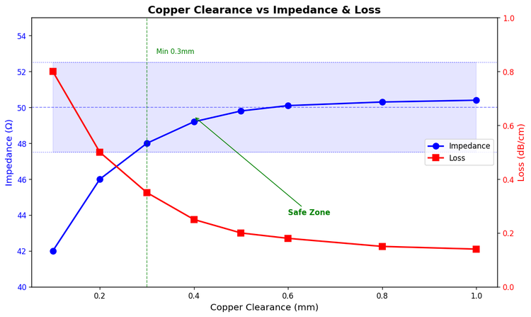
Figure 2: Influence of Copper Clearance on Impedance and Loss
[Note] For general RF lines such as 2.4GHz and 5GHz, it is a common practice to reserve a clearance area of 0.2-0.5mm on both sides. Below 0.2mm, both impedance and loss will deteriorate significantly.
Personally, if you need to precisely control the impedance, you should determine the spacing through simulation during the design phase, rather than pouring copper by feeling.
When Copper Pouring Is Prohibited
Some areas are "copper-pouring prohibited areas" and must be kept clear:
- Below crystal oscillators and clock circuits: Copper pouring is prohibited within at least 0.3mm to prevent crosstalk and radiation.
- Around antennas and matching networks: Strictly reserve clearance areas according to the reference design, and the matching network area must also be kept "clean".
- High-impedance nodes: Such as filter input and output nodes, keep clearance around to avoid parasitic capacitance affecting the filtering effect.
"Stitching" Skills of Ground Vias
Copper pouring must be connected to the GND network. Suspended "isolated copper" will become an antenna, receiving and radiating noise.
The solution is to use via stitching to connect the GND copper skins of different layers at multiple points to form a low-impedance "ground wall". The via spacing is recommended to be less than 1/20 of the wavelength of the highest operating frequency.
For example: 2.4GHz signal, wavelength is about 125mm, λ/20 is about 6mm. So it is safe to control the ground via spacing within 5mm.
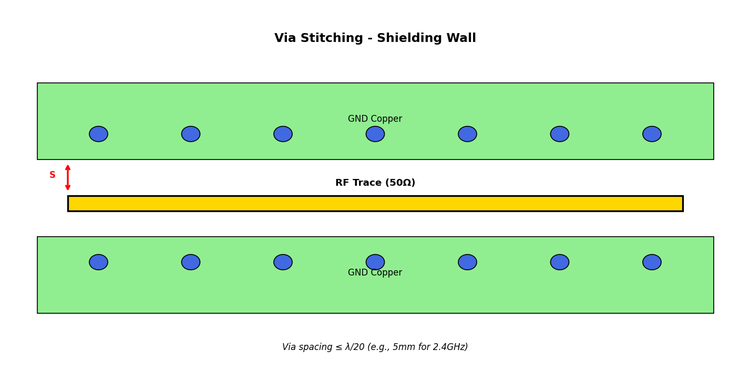
Figure 3: Schematic Diagram of Ground Via Shielding Wall
Practical Design Points
Combined with my experience, I summarize several practical design points:
1. Impedance Control First
Impedance control of RF traces is the top priority. First, use an impedance calculation tool (such as SI9000) to calculate the line width, and then verify it through electromagnetic simulation software (such as ADS, HFSS). Keep the line width uniform during design and avoid sudden changes.
Make arc chamfers at the transition between the microstrip line and the device pins, with a radius ≥0.5mm, to reduce impedance discontinuity.
2. Complete Reference Ground Plane
The ground plane adjacent to the RF signal layer must be complete, without slots or hollowing. Any cutting will damage the return path and cause impedance discontinuity.
[Example] A WiFi module has a 1mm-wide slot in the ground plane under the microstrip line. The measured impedance suddenly changed from 50Ω to 55Ω, and the return loss deteriorated from -18dB to -12dB. It returned to normal after removing the slot.
3. Reasonable Planning of Copper Clearance
The copper clearance on both sides of RF traces follows the following principles:
- Conventional RF lines (≤6GHz): ≥0.3mm
- High-frequency RF lines (6-10GHz): ≥0.4mm
- Millimeter waves (>10GHz): It is recommended not to perform side copper pouring, or determine according to simulation results
4. Dense Arrangement of Ground Vias
Use dense ground vias around RF modules and on both sides of key signal lines to form a "shielding wall". Via spacing ≤λ/20, and can be denser for high-frequency applications.
The spacing between vias and signal lines is recommended to be 1-3 times the line width, which can provide good shielding without affecting impedance.
5. Indispensable Simulation Verification
For high-speed and high-frequency designs, do not rely entirely on experience. Use electromagnetic simulation tools to check impedance matching, crosstalk, and radiation performance. Especially the influence of copper clearance can be seen at a glance through simulation.
[Recommendation] After completing the design, perform an S-parameter simulation. Check whether S11 (return loss) meets the requirements in the operating frequency band and whether S21 (insertion loss) is within the expected range. Finding problems early and modifying them is much lower in cost than modifying after board production.
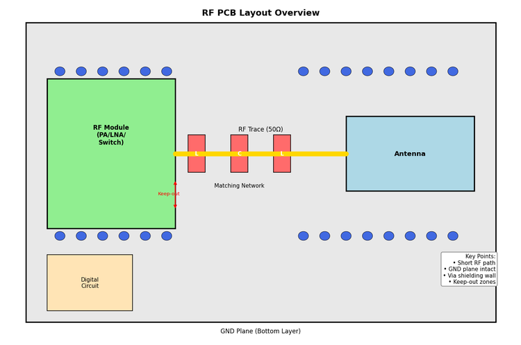
Figure 4: Schematic Diagram of RF PCB Layout Key Points
Clarification of Common Misunderstandings
Finally, let’s clarify several common misunderstandings:
Misunderstanding 1: "The more copper poured, the better"
Wrong! Blind copper pouring in the RF area will change impedance and increase loss. Copper pouring must be strategic, and clearance must be reserved where necessary.
Misunderstanding 2: "Ground vias can be placed randomly"
Wrong! The position and spacing of ground vias are particular. Too dense will increase processing costs, and too sparse will result in insufficient shielding effect. Arranging according to the λ/20 principle is reasonable.
Misunderstanding 3: "50Ω impedance is enough"
Not completely correct. Impedance control accuracy is also very important. ±5% is the basic requirement, and ±3% for high-frequency applications. Consider process deviations during design and leave a margin.
Summary
The difficulty of tuning the RF front-end is often not a component problem, but the PCB design details are not in place. Impedance matching and copper clearance, these two "hidden parameters" often determine the success or failure of RF performance.
Remember these core points:
- Impedance matching is the foundation: Return loss ≤-15dB, VSWR ≤1.5, control accuracy ±5%
- Reasonable copper clearance: Reserve 0.2-0.5mm clearance on both sides of RF lines, prohibit copper pouring in sensitive areas
- Complete ground plane: No cutting in the ground plane under RF traces
- Rule-based stitching vias: Spacing ≤λ/20 to form a low-impedance ground wall
- Indispensable simulation verification: Perform S-parameter simulation before board production, find and modify problems early
There are no shortcuts to RF design, but mastering these points can at least avoid the most common pitfalls. I hope these experiences are helpful to you.
About Maxipcb
Maxipcb empowers innovators to turn cutting-edge technologies into reality.
We offer one-stop solutions for design, simulation, testing, PCB manufacturing, component procurement and SMT assembly, enabling efficient development, rapid deployment and risk control across the full product lifecycle.Serving the world in communications, industrial automation, aerospace, automotive, semiconductor and beyond, we build a safer, more connected future together.
