In a high‑speed printed circuit board (PCB), vias have long been criticised for degrading signal‑integrity performance. However, the use of vias is unavoidable. On a standard board, components are placed on the top layer, while the differential‑pair traces are routed on internal layers. Internal layers offer lower electromagnetic radiation and lower pair‑to‑pair crosstalk. Vias must be used to connect the components on the board plane to the internal layers.
In a high‑speed printed circuit board (PCB), vias have long been criticised for degrading signal‑integrity performance. However, the use of vias is unavoidable. On a standard board, components are placed on the top layer, while the differential‑pair traces are routed on internal layers. Internal layers offer lower electromagnetic radiation and lower pair‑to‑pair crosstalk. Vias must be used to connect the components on the board plane to the internal layers.
Fortunately, it is possible to design a transparent via that minimises the impact on performance. In this blog post, I will discuss:
-
Basic via components
-
Electrical properties of vias
-
A method for building a transparent via
-
Test results for a differential via structure
1. Basics of Via Structures
Let us start by examining the components of a simple via that connects a top‑layer transmission line to an internal layer. Figure 1 is a 3D illustration showing the via structure. There are four basic components: the signal via, the via stub, the via pad, and the anti‑pad.
The via is the metal cylinder plated on the outside of the hole drilled through the board between the top and bottom layers. The signal via connects the transmission lines on different layers. The via stub is the unused portion of the via. The via pad is the annular ring that connects the via to the top or internal transmission line. The anti‑pad is the annular clearance hole in each power or ground layer to prevent short circuits to the power and ground planes.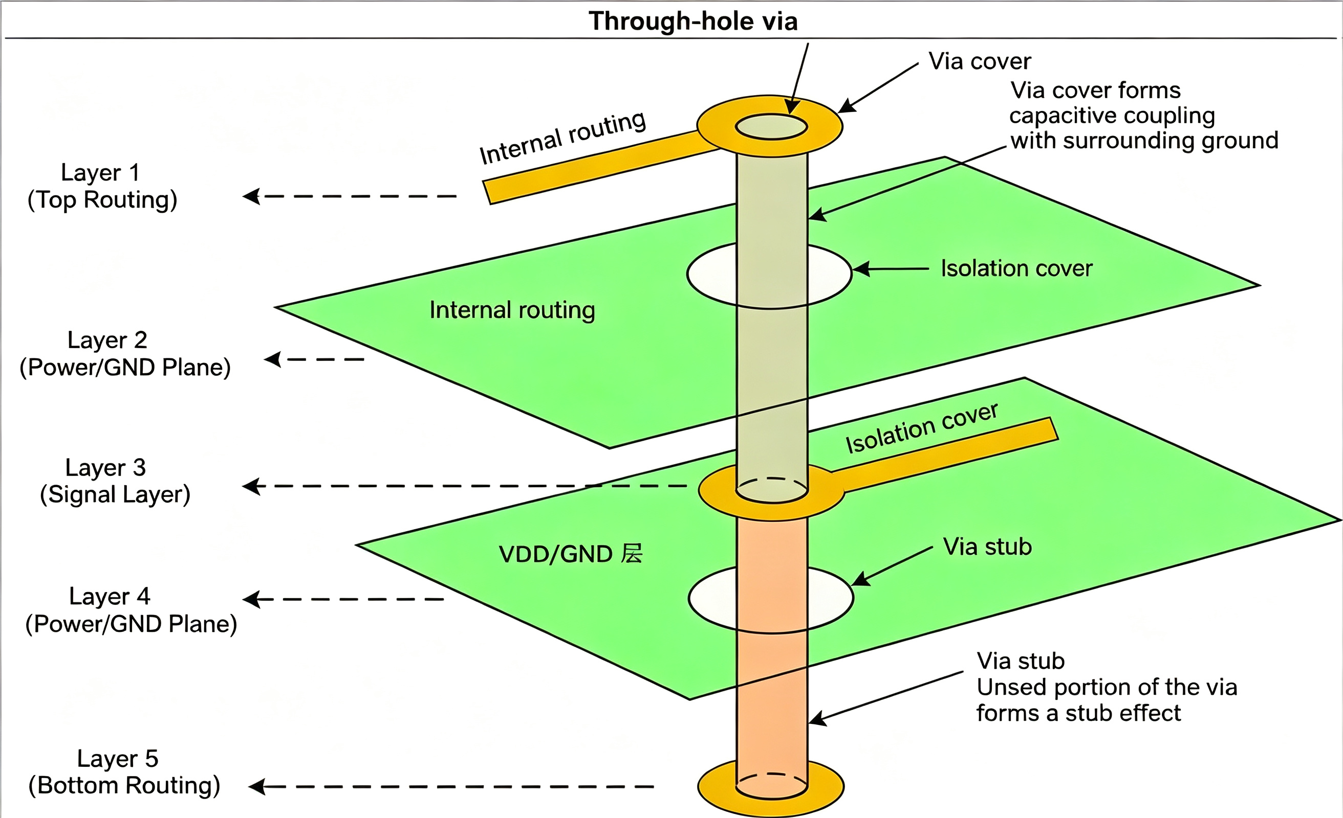
Figure 1: 3D illustration of a single via
2. Electrical Properties of Via Components
Let us take a closer look at the electrical properties of each via component, as shown in Table 1.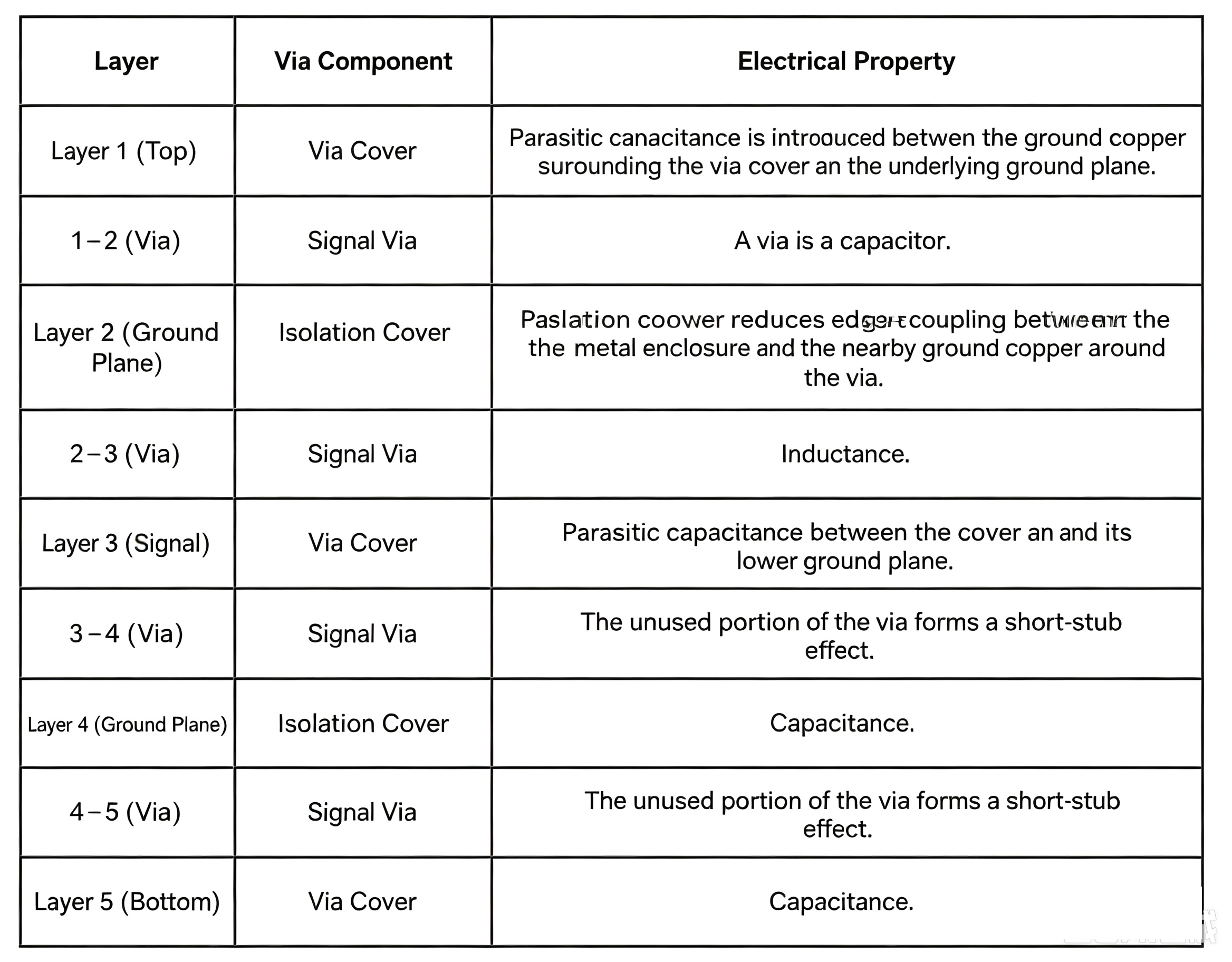
Table 1: Electrical properties of the via components shown in Figure 1
A simple via is a series of π‑type networks, consisting of C‑L‑C (capacitance‑inductance‑capacitance) elements formed between two adjacent layers. Table 2 shows the effects of via dimensions.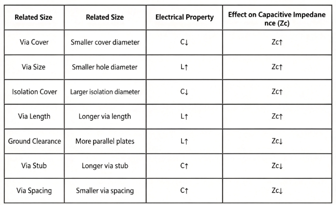
Table 2: Visual effects of via dimensions
By balancing the inductance and parasitic capacitance, it is possible to design a via with the same characteristic impedance as the transmission line, so that it does not have a noticeable effect on board operation. There is no simple formula for converting via dimensions into C and L elements. A 3D electromagnetic (EM) field solver can predict the structure's impedance based on the dimensions used in the PCB layout. By iteratively adjusting the structure dimensions and running 3D simulations, the via dimensions can be optimised to achieve the desired impedance and bandwidth requirements.
3. Designing a Transparent Differential Via
As we discussed in a previous post, when implementing a differential pair, there must be a high degree of symmetry between line A and line B. These pairs are routed on the same layer. If a via is required, vias must be placed close to each other on both lines. Because the two vias of the differential pair are close together, a single shared oval anti‑pad can be used for the two vias to reduce parasitic capacitance, rather than using two separate anti‑pads. Ground vias are also placed next to each via so that they can provide ground return paths for the A and B vias.
Figure 2 shows an example of a ground‑signal‑signal‑ground (GSSG) differential via structure. The distance between the two adjacent vias is called the via pitch. The smaller the via pitch, the greater the mutual coupling capacitance.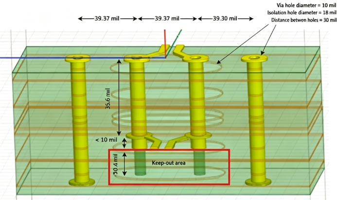
Figure 2: GSSG differential via with back drilling
Do not forget that at data rates above 10 Gbps, via stubs can severely affect high‑speed signal integrity. Fortunately, there is a PCB manufacturing process called back drilling, which removes the unused via barrel. Depending on manufacturing tolerances, back drilling removes the unused via metal and reduces the via stub to less than 10 mils.
A 3D EM simulator is used to design the differential via according to the required impedance and bandwidth. This is an iterative process, adjusting the via dimensions and running EM simulations repeatedly until the desired impedance and bandwidth are achieved.
4. How to Verify Performance
The differential via design shown in Figure 2 was built and tested. The test coupon included a pair of differential traces on the top layer, followed by differential vias to internal differential traces, and then a second pair of differential vias connecting back to the top layer to ball‑grid array (BGA) landing pads. The total signal path length was approximately 1330 mils. Differential impedance was measured using a differential time‑domain reflectometer (TDR), bandwidth was measured with a network analyser, and a high‑speed oscilloscope was used to measure data eye diagrams to understand the impact on the signal. Figures 3, 4, and 5 show the impedance, bandwidth, and eye diagrams, respectively. The left side shows test results with back drilling, while the right side shows results without back drilling. In the bandwidth Bode plot of Figure 5, it is very clear that back drilling is essential for achieving high performance at data rates greater than 10 Gbps.
With back drilling, ZDIFF ≈ 85 Ω. Without back drilling, ZDIFF ≈ 58 Ω.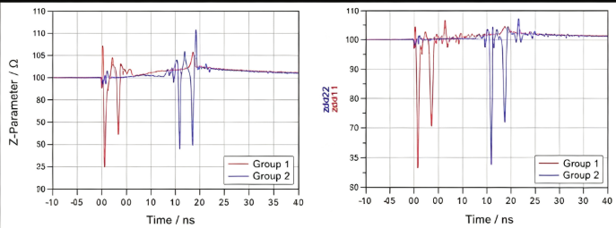
Figure 3: TDR impedance Bode plot
Insertion loss at 12.5 GHz ≈ 3 dB (with back drilling); insertion loss at 12.5 GHz > 8 dB (without back drilling).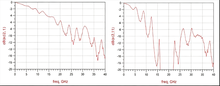
Figure 4: Frequency response
With back drilling, the data eye is open. Without back drilling, the data eye is closed.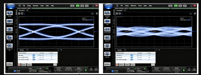
Figure 5: Data eye diagram at 25 Gbps
TI offers a rich library of high‑speed signal‑conditioning integrated circuits (ICs), such as retimers and redrivers. These help mitigate and compensate for the imperfections and high insertion loss of all types of differential pairs, enabling reliable data communication and extending transmission distances in advanced systems.
Please leave a comment below – I would love to hear your feedback on this post or suggestions for what you would like to see in future "Differential Pair" posts.
Other Resources
-
View the TI low‑voltage differential signalling (LVDS), multi‑point LVDS (MLVDS), and signal‑conditioning retimer and redriver product library overviews.
-
Learn more about differential signalling from the LVDS Owner's Manual.
-
Read the TI two‑port 40‑gigabit Ethernet (40GbE)/10GbE quad small form‑factor pluggable (QSFP+) signal conditioner reference design.
-
Learn about TI's peripheral component interconnect express (PCIe) Gen‑3 board from the DS80PCI810 linear redriver reference design.
About Maxipcb
Maxipcb empowers innovators to turn cutting-edge technologies into reality.We offer one-stop solutions for design, simulation, testing, PCB manufacturing, component procurement and SMT assembly, enabling efficient development, rapid deployment and risk control across the full product lifecycle.
Serving the world in communications, industrial automation, aerospace, automotive, semiconductor and beyond, we build a safer, more connected future together.
