FPGAs are devices that provide numerous logic cells and other features such as transceivers, PLLs, and MAC units for complex processing tasks. FPGAs have become very powerful, and effectively powering them is a critical aspect of the design that is often underestimated.
Introduction
FPGAs are devices that provide numerous logic cells and other features such as transceivers, PLLs, and MAC units for complex processing tasks. FPGAs have become very powerful, and effectively powering them is a critical aspect of the design that is often underestimated.
This article analyses the power requirements for FPGAs, provides guidance on how and where to place the power supply on the PCB, and walks the reader through the design steps using an example in which the FPGA is powered from a 12 V bus – the main output from a mains‑fed SMPS.
Power Estimators and Voltage Requirements
An important aspect of FPGA design is determining the required voltage levels and the current requirements for each voltage rail. Major FPGA vendors provide comprehensive calculators to help determine these requirements, taking into account factors such as operating frequency, the number of gates used, and their switching rates. For example, Altera offers the PowerPlay Early Power Estimator, and Xilinx provides the XPower Analyzer.
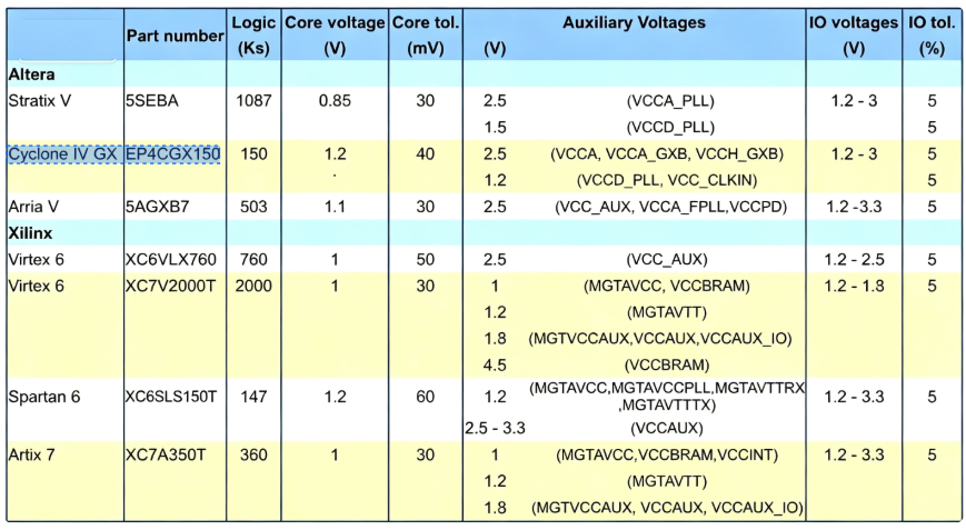
Table 1 lists some typical voltage rails required by Altera and Xilinx devices, grouped into three core voltages: I/O voltage, transceiver voltage, and auxiliary voltage.
POL and Power Distribution Systems
FPGAs with lower core voltages require high current, high accuracy, and minimal ripple. To achieve this, decoupling capacitors should be placed as close as possible to the FPGA to minimise the ESR and ESL in the decoupling path.
It is also good practice to place the POL regulator as close as possible to the device, without interfering with the FPGA's I/O paths. Higher operating frequencies, together with integrated controllers, drivers, and MOSFETs, help achieve a compact layout. A small solution footprint allows the regulator to be placed close to the FPGA, improving transient response. Figure 1 shows an example of a 3 A regulator from the Vishay microBUCK product family.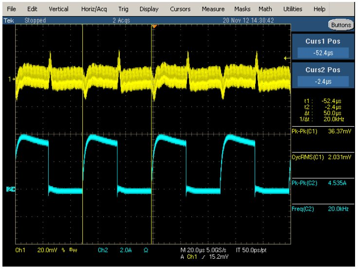
Figure 1: Step response of the SiP12107
VIN = 5 V, VOUT = 1.2 V, Fsw = 2 MHz; load step = 0‑3 A at 20 kHz; L = 330 nH, CIN = 22 μF, COUT = 22 μF; yellow = VOUT, blue = current.
As can be seen, with minimum input and output capacitance of 22 μF (0805), the step response is 37 mV peak‑to‑peak (with additional capacitance on the load).
The regulator uses a current‑mode constant‑on‑time (CM‑COT) topology and does not require external ripple injection for stability. This helps reduce component count and provides excellent transient response.
Selecting the Right Regulator
When selecting a regulator, one of the primary criteria is the required input operating voltage. Next, the current requirement should be examined. After the final list of candidate devices is established, other characteristics – such as operating frequency range and light‑load power‑saving modes – should be checked, allowing the designer to determine the most suitable device for the application.
Many switching regulator suppliers now offer online simulation tools to aid power supply design. For example, Vishay regulators are supported by the PowerCAD online simulation tool. After analysing the available options using the method described above, the online simulator allows the user to quickly complete a design (see the simulation schematic in Figure 2). Once this step is complete, operating waveforms such as startup, step response, and steady‑state operation can be examined to understand current and voltage levels. The simulator also features efficiency analysis, detailed loss breakdown for all components, and a BOM generator.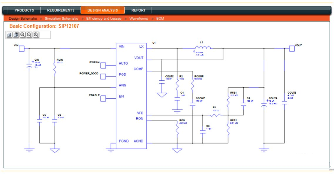
Figure 2: Vishay PowerCAD software simulation schematic
Initial Design Example
Let us take as an example a Cyclone IV EP4CGX75 with a clock speed of 362 MHz.
-
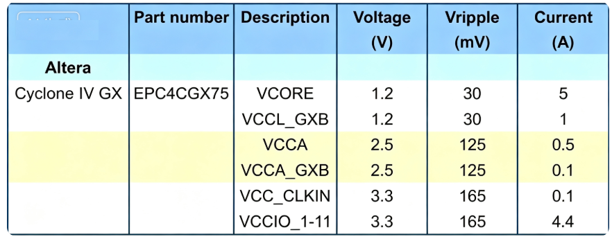
Use PowerPlay to determine the current requirements for each power rail. In this example, we analyse only the FPGA supply with the worst‑case load on the outputs. Table 2 lists the design specifications obtained from the early estimator software.
-
Now the devices can be selected. From Table 2, it can be seen that the core voltage is 1.2 V at 5 A. There is also an additional 1 A requirement from this rail, bringing the total current requirement from this rail to 6 A. The other two voltages follow the same pattern, leading to the power architecture shown in Figure 3.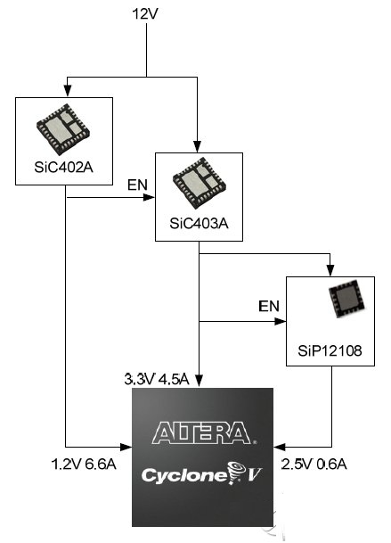
Figure 3: Example solution
-
Run the Vishay PowerCAD simulator to obtain the results shown in Table 3.

The efficiency results from these simulations differ by less than 1 % from the final design. Although they cannot replace a thorough design process, they help designers quickly understand the likely outcome before committing time and effort to hardware design.
Author: Owain Bryant, Product Application Engineer, Vishay Siliconix
About Maxipcb
Maxipcb empowers innovators to turn cutting-edge technologies into reality.We offer one-stop solutions for design, simulation, testing, PCB manufacturing, component procurement and SMT assembly, enabling efficient development, rapid deployment and risk control across the full product lifecycle.
Serving the world in communications, industrial automation, aerospace, automotive, semiconductor and beyond, we build a safer, more connected future together.
