Transmission lines are used to transmit signals or electrical energy from one point to another. Familiar examples include overhead power lines on streets, telephone lines, and the interconnections between components on PCBs in electronic technology.
Transmission Lines Become Circuit Elements
Transmission lines are used to transmit signals or electrical energy from one point to another. Familiar examples include overhead power lines on streets, telephone lines, and the interconnections between components on PCBs in electronic technology. In basic circuit analysis, it is assumed that the length of transmission lines between components is negligible, so that connections can be represented by topological diagrams. Under this assumption, the time measured at the source is considered the same as the time measured at any point in the circuit – there is no signal delay, and the phase difference of sinusoidal waveforms is zero.
When the distance between the source and the load becomes sufficiently large, the time‑delay effect becomes significant, and the phase difference between sinusoidal waveforms measured at the source and load at the same instant can be observed.
For the basic components – resistors, capacitors, and inductors – in lumped‑parameter theory, the transmission time delay across the component is negligible. However, when their physical dimensions become large enough, or when the connecting lines are sufficiently long, they must be treated as distributed‑parameter components. This means that the resistance, capacitance, and inductance parameters must be calculated on a per‑unit‑length basis.
When a transmission line is long enough, it exhibits distributed‑parameter characteristics, and thus the transmission line itself becomes a circuit element.
Construction of a Transmission Line Circuit
Line Self‑Inductance
Regardless of the shape of the transmission line, when current I flows through it, a magnetic flux Φ is generated, which in turn produces self‑inductance:

For engineering practitioners, this result can be used directly. Therefore, when high‑frequency signals pass through the line, the inductive reactance generated becomes significant and cannot be ignored.
Capacitance Between Transmission Lines
Consider two infinitely long transmission lines consisting of two parallel cylindrical conductors carrying opposite charges. Assuming one conductor is at zero potential, and the other is a cylindrical conductor of radius b at potential V, with an axial separation h between them, the capacitance between them is:

The capacitance depends only on the line length L, the separation h, and the conductor radius b – it is independent of the voltage between the conductors.
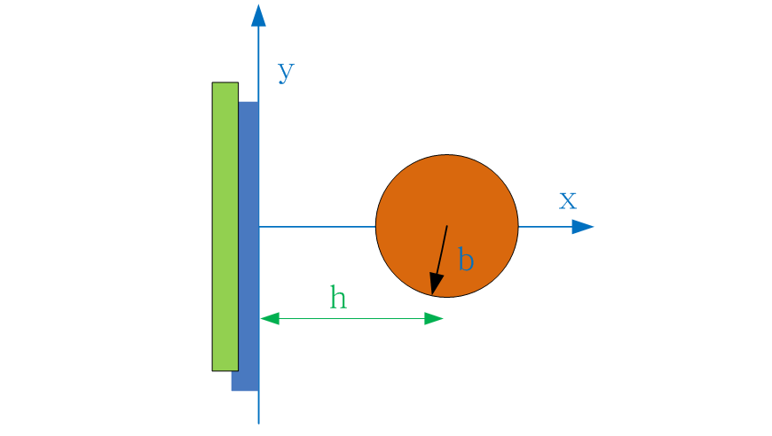
For a conductor of length L, the smaller the distance to a zero‑potential conductive plane, the larger the capacitance – a characteristic consistent with parallel‑plate capacitance. Since capacitance increases with more parallel connections, if there are N conductors of length L, the total inter‑conductor capacitance is magnified N times.
The potential difference between conductors affects the equivalent line charge density:

This capacitance formula is very important. If the transmission line is divided into segments of length L, each segment has a capacitance C. Multiple segments of length L are connected in parallel, so the longer the line, the greater the inter‑line capacitance. From the formula, it can also be seen that the larger the line spacing, the smaller the capacitance, and the smaller the wire diameter, the smaller the capacitance.
To understand this principle, consider the limiting cases: if the line spacing is infinitely large, the capacitance tends to zero; if the wire diameter is infinitely small (almost invisible), the capacitance also tends to zero. For a long conductor L, as L tends to infinity, the capacitance tends to infinity.
This provides practical guidance for engineering: for high‑frequency signal lines, every effort should be made to reduce line length and increase the clearance between the line and ground. Do not place a digital ground plane beneath high‑frequency signals. Signal lines should use the minimum trace width – currently, 6‑mil trace widths are achievable with standard PCB manufacturing processes, and some PCB manufacturers can achieve 4‑mil widths.
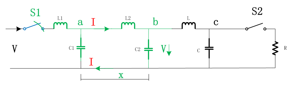
Using lumped capacitance and lumped inductance, a given transmission line can be modelled as follows:
Signal Propagation in Transmission Lines
Assume an ideal lossless transmission line where all input power is eventually delivered to the output.
At time t = 0, switch S1 is closed, and voltage V is applied to the input of the transmission line. At the instant the switch closes, the voltage V cannot appear instantaneously at all points along the line – it propagates from the input towards the load at a finite velocity.
In the figure above, green indicates the portion of the transmission line that has already been charged to voltage V, while black indicates the remaining portion that has not yet been charged.
As the transmission line charges, the signal wave propagates from left to right at velocity v. When the wave reaches the load end, all or part of the voltage and current waves are reflected. The magnitude of the reflection depends on the termination characteristics at the load.
-
If the terminating resistor is disconnected, no energy is dissipated at the load, and the entire voltage wave is reflected back.
-
If the terminating resistor is connected, part or all of the energy is dissipated, and only part (or none) of the incident voltage is reflected.
Operation of Elements in the Transmission Line Model
Case 1: Switch S1 Closed, Switch S2 Open
When switch S1 is closed, the current in L1 begins to increase, and C1 begins to charge. After C1 is fully charged, current in L2 begins to increase, followed by C2 charging, and so on sequentially until all capacitors are fully charged.
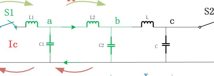
The speed of signal wave propagation depends not only on how quickly the current in each inductor reaches its maximum, but also on how quickly the voltage across each capacitor reaches its maximum. If the values of L and C are small, the wave propagates faster.
It can be shown that the wave velocity is inversely proportional to a function determined by the product of inductance and capacitance:

Case 2: Switch S1 Closed, Switch S2 Closed
When a resistor is connected to the output of a fully charged transmission line, the capacitor C closest to the resistor R discharges first through the resistor, while the inductor generates a back‑EMF. Then C2 discharges, followed by C1. When all capacitors have discharged, a voltage spike appears across the resistor.
Transmission Line Circuit Model
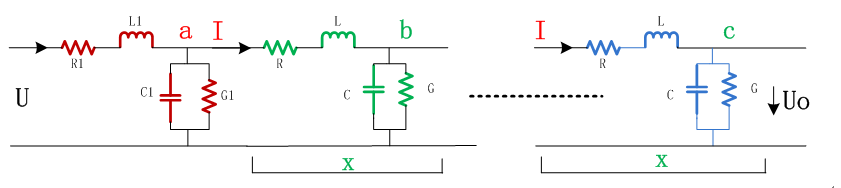
A transmission line should also include a series resistance R, which is related to the conductivity of the conductor. Lower‑conductivity conductors have higher resistance and correspondingly higher losses.
In addition, a shunt conductance G should be included, representing the leakage current flowing through the dielectric between the transmission lines. Higher dielectric conductivity results in greater leakage current and larger G.
Both series resistance R and shunt conductance G are functions of frequency. Thus, we obtain the transmission line circuit model:
About Maxipcb
Maxipcb empowers innovators to turn cutting-edge technologies into reality.We offer one-stop solutions for design, simulation, testing, PCB manufacturing, component procurement and SMT assembly, enabling efficient development, rapid deployment and risk control across the full product lifecycle.
Serving the world in communications, industrial automation, aerospace, automotive, semiconductor and beyond, we build a safer, more connected future together.

